CSS02 Simulation

SIR, SEIR - Compartmental Model

Reference

1. https://scipython.com/book/chapter-8-scipy/additional-examples/the-sir-epidemic-model/

2. https://python.quantecon.org/sir_model.html

import numpy as np
from scipy.integrate import odeint
import matplotlib.pyplot as plt

# Total population, N.
N = 1000
# Initial number of infected and recovered individuals, I0 and R0.
I0, R0 = 1, 0
# Everyone else, S0, is susceptible to infection initially.
S0 = N - I0 - R0
# Contact rate, beta, and mean recovery rate, gamma, (in 1/days).
beta, gamma = 0.2, 1./10 

np.linespace():

• https://numpy.org/doc/stable/reference/generated/numpy.linspace.html

• Return evenly spaced numbers over a specified interval.

• Returns num evenly spaced samples, calculated over the interval [start, stop].

• The endpoint of the interval can optionally be excluded.

# A grid of time points (in days)
t = np.linspace(0, 160, 160)
t

array([  0.        ,   1.00628931,   2.01257862,   3.01886792,
         4.02515723,   5.03144654,   6.03773585,   7.04402516,
         8.05031447,   9.05660377,  10.06289308,  11.06918239,
        12.0754717 ,  13.08176101,  14.08805031,  15.09433962,
        16.10062893,  17.10691824,  18.11320755,  19.11949686,
        20.12578616,  21.13207547,  22.13836478,  23.14465409,
        24.1509434 ,  25.1572327 ,  26.16352201,  27.16981132,
        28.17610063,  29.18238994,  30.18867925,  31.19496855,
        32.20125786,  33.20754717,  34.21383648,  35.22012579,
        36.22641509,  37.2327044 ,  38.23899371,  39.24528302,
        40.25157233,  41.25786164,  42.26415094,  43.27044025,
        44.27672956,  45.28301887,  46.28930818,  47.29559748,
        48.30188679,  49.3081761 ,  50.31446541,  51.32075472,
        52.32704403,  53.33333333,  54.33962264,  55.34591195,
        56.35220126,  57.35849057,  58.36477987,  59.37106918,
        60.37735849,  61.3836478 ,  62.38993711,  63.39622642,
        64.40251572,  65.40880503,  66.41509434,  67.42138365,
        68.42767296,  69.43396226,  70.44025157,  71.44654088,
        72.45283019,  73.4591195 ,  74.46540881,  75.47169811,
        76.47798742,  77.48427673,  78.49056604,  79.49685535,
        80.50314465,  81.50943396,  82.51572327,  83.52201258,
        84.52830189,  85.53459119,  86.5408805 ,  87.54716981,
        88.55345912,  89.55974843,  90.56603774,  91.57232704,
        92.57861635,  93.58490566,  94.59119497,  95.59748428,
        96.60377358,  97.61006289,  98.6163522 ,  99.62264151,
       100.62893082, 101.63522013, 102.64150943, 103.64779874,
       104.65408805, 105.66037736, 106.66666667, 107.67295597,
       108.67924528, 109.68553459, 110.6918239 , 111.69811321,
       112.70440252, 113.71069182, 114.71698113, 115.72327044,
       116.72955975, 117.73584906, 118.74213836, 119.74842767,
       120.75471698, 121.76100629, 122.7672956 , 123.77358491,
       124.77987421, 125.78616352, 126.79245283, 127.79874214,
       128.80503145, 129.81132075, 130.81761006, 131.82389937,
       132.83018868, 133.83647799, 134.8427673 , 135.8490566 ,
       136.85534591, 137.86163522, 138.86792453, 139.87421384,
       140.88050314, 141.88679245, 142.89308176, 143.89937107,
       144.90566038, 145.91194969, 146.91823899, 147.9245283 ,
       148.93081761, 149.93710692, 150.94339623, 151.94968553,
       152.95597484, 153.96226415, 154.96855346, 155.97484277,
       156.98113208, 157.98742138, 158.99371069, 160.        ])

SIR Model

• https://scipython.com/book/chapter-8-scipy/additional-examples/the-sir-epidemic-model/

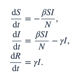
# The SIR model differential equations.
def deriv(y, t, N, beta, gamma):
    S, I, R = y
    dSdt = -beta * S * I / N
    dIdt = beta * S * I / N - gamma * I
    dRdt = gamma * I
    return dSdt, dIdt, dRdt

odeint()

y = odeint(model, y0, t)

1. model: Function name that returns derivative values at requested y and t values as dydt = model(y,t)

2. y0: Initial conditions of the differential states

3. t: Time points at which the solution should be reported. Additional internal points are often calculated to maintain accuracy of the solution but are not reported.

Reference:

• https://docs.scipy.org/doc/scipy/reference/generated/scipy.integrate.odeint.html

# Initial conditions vector
y0 = S0, I0, R0
# Integrate the SIR equations over the time grid, t.
ret = odeint(deriv, y0, t, args=(N, beta, gamma))
S, I, R = ret.T

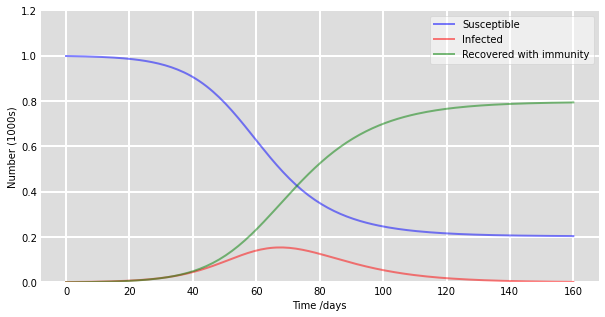
# Plot the data on three separate curves for S(t), I(t) and R(t)
fig = plt.figure(facecolor='w', figsize=(10, 5))
ax = fig.add_subplot(111, facecolor='#dddddd', axisbelow=True)
ax.plot(t, S/1000, 'b', alpha=0.5, lw=2, label='Susceptible')
ax.plot(t, I/1000, 'r', alpha=0.5, lw=2, label='Infected')
ax.plot(t, R/1000, 'g', alpha=0.5, lw=2, label='Recovered with immunity')
ax.set_xlabel('Time /days')
ax.set_ylabel('Number (1000s)')
ax.set_ylim(0,1.2)
ax.yaxis.set_tick_params(length=0)
ax.xaxis.set_tick_params(length=0)

ax.grid(which='major', c='w', lw=2, ls='-')
legend = ax.legend()
legend.get_frame().set_alpha(0.5)
for spine in ('top', 'right', 'bottom', 'left'):
    ax.spines[spine].set_visible(False)
plt.show()