Bokeh & Seaborn(Vaccinating)#
Main Reference: https://pandas.pydata.org/pandas-docs/stable/user_guide/visualization.html
用來做範例的這個資料是COVID疫情期間的各國疫苗接種資料。資料包含不同國家在不同日期所上傳的資料。要注意的是,這份資料的空值相當的多,有看得出來是空值的資料(如某些項目沒有填寫),也有沒有填寫的天數。每個國家開始登記的日期、漏登的日期、後來不再追蹤的日期都不一定,因此對齊資料的日期、決定資料可回答問題的區間都非常辛苦。
Load vaccination data#
import pandas as pd
raw = pd.read_csv("https://raw.githubusercontent.com/owid/covid-19-data/master/public/data/owid-covid-data.csv")
/Users/jirlong/opt/anaconda3/lib/python3.9/site-packages/pandas/core/computation/expressions.py:21: UserWarning: Pandas requires version '2.8.4' or newer of 'numexpr' (version '2.8.1' currently installed).
  from pandas.core.computation.check import NUMEXPR_INSTALLED
/Users/jirlong/opt/anaconda3/lib/python3.9/site-packages/pandas/core/arrays/masked.py:60: UserWarning: Pandas requires version '1.3.6' or newer of 'bottleneck' (version '1.3.4' currently installed).
  from pandas.core import (
---------------------------------------------------------------------------
KeyboardInterrupt                         Traceback (most recent call last)
Input In [1], in <cell line: 2>()
      1 import pandas as pd
----> 2 raw = pd.read_csv("https://raw.githubusercontent.com/owid/covid-19-data/master/public/data/owid-covid-data.csv")

File ~/opt/anaconda3/lib/python3.9/site-packages/pandas/io/parsers/readers.py:1026, in read_csv(filepath_or_buffer, sep, delimiter, header, names, index_col, usecols, dtype, engine, converters, true_values, false_values, skipinitialspace, skiprows, skipfooter, nrows, na_values, keep_default_na, na_filter, verbose, skip_blank_lines, parse_dates, infer_datetime_format, keep_date_col, date_parser, date_format, dayfirst, cache_dates, iterator, chunksize, compression, thousands, decimal, lineterminator, quotechar, quoting, doublequote, escapechar, comment, encoding, encoding_errors, dialect, on_bad_lines, delim_whitespace, low_memory, memory_map, float_precision, storage_options, dtype_backend)
   1013 kwds_defaults = _refine_defaults_read(
   1014     dialect,
   1015     delimiter,
   (...)
   1022     dtype_backend=dtype_backend,
   1023 )
   1024 kwds.update(kwds_defaults)
-> 1026 return _read(filepath_or_buffer, kwds)

File ~/opt/anaconda3/lib/python3.9/site-packages/pandas/io/parsers/readers.py:620, in _read(filepath_or_buffer, kwds)
    617 _validate_names(kwds.get("names", None))
    619 # Create the parser.
--> 620 parser = TextFileReader(filepath_or_buffer, **kwds)
    622 if chunksize or iterator:
    623     return parser

File ~/opt/anaconda3/lib/python3.9/site-packages/pandas/io/parsers/readers.py:1620, in TextFileReader.__init__(self, f, engine, **kwds)
   1617     self.options["has_index_names"] = kwds["has_index_names"]
   1619 self.handles: IOHandles | None = None
-> 1620 self._engine = self._make_engine(f, self.engine)

File ~/opt/anaconda3/lib/python3.9/site-packages/pandas/io/parsers/readers.py:1880, in TextFileReader._make_engine(self, f, engine)
   1878     if "b" not in mode:
   1879         mode += "b"
-> 1880 self.handles = get_handle(
   1881     f,
   1882     mode,
   1883     encoding=self.options.get("encoding", None),
   1884     compression=self.options.get("compression", None),
   1885     memory_map=self.options.get("memory_map", False),
   1886     is_text=is_text,
   1887     errors=self.options.get("encoding_errors", "strict"),
   1888     storage_options=self.options.get("storage_options", None),
   1889 )
   1890 assert self.handles is not None
   1891 f = self.handles.handle

File ~/opt/anaconda3/lib/python3.9/site-packages/pandas/io/common.py:728, in get_handle(path_or_buf, mode, encoding, compression, memory_map, is_text, errors, storage_options)
    725     codecs.lookup_error(errors)
    727 # open URLs
--> 728 ioargs = _get_filepath_or_buffer(
    729     path_or_buf,
    730     encoding=encoding,
    731     compression=compression,
    732     mode=mode,
    733     storage_options=storage_options,
    734 )
    736 handle = ioargs.filepath_or_buffer
    737 handles: list[BaseBuffer]

File ~/opt/anaconda3/lib/python3.9/site-packages/pandas/io/common.py:389, in _get_filepath_or_buffer(filepath_or_buffer, encoding, compression, mode, storage_options)
    386         if content_encoding == "gzip":
    387             # Override compression based on Content-Encoding header
    388             compression = {"method": "gzip"}
--> 389         reader = BytesIO(req.read())
    390     return IOArgs(
    391         filepath_or_buffer=reader,
    392         encoding=encoding,
   (...)
    395         mode=fsspec_mode,
    396     )
    398 if is_fsspec_url(filepath_or_buffer):

File ~/opt/anaconda3/lib/python3.9/http/client.py:476, in HTTPResponse.read(self, amt)
    474 else:
    475     try:
--> 476         s = self._safe_read(self.length)
    477     except IncompleteRead:
    478         self._close_conn()

File ~/opt/anaconda3/lib/python3.9/http/client.py:626, in HTTPResponse._safe_read(self, amt)
    624 s = []
    625 while amt > 0:
--> 626     chunk = self.fp.read(min(amt, MAXAMOUNT))
    627     if not chunk:
    628         raise IncompleteRead(b''.join(s), amt)

File ~/opt/anaconda3/lib/python3.9/socket.py:704, in SocketIO.readinto(self, b)
    702 while True:
    703     try:
--> 704         return self._sock.recv_into(b)
    705     except timeout:
    706         self._timeout_occurred = True

File ~/opt/anaconda3/lib/python3.9/ssl.py:1241, in SSLSocket.recv_into(self, buffer, nbytes, flags)
   1237     if flags != 0:
   1238         raise ValueError(
   1239           "non-zero flags not allowed in calls to recv_into() on %s" %
   1240           self.__class__)
-> 1241     return self.read(nbytes, buffer)
   1242 else:
   1243     return super().recv_into(buffer, nbytes, flags)

File ~/opt/anaconda3/lib/python3.9/ssl.py:1099, in SSLSocket.read(self, len, buffer)
   1097 try:
   1098     if buffer is not None:
-> 1099         return self._sslobj.read(len, buffer)
   1100     else:
   1101         return self._sslobj.read(len)

KeyboardInterrupt:
raw
| iso_code | continent | location | date | total_cases | new_cases | new_cases_smoothed | total_deaths | new_deaths | new_deaths_smoothed | ... | male_smokers | handwashing_facilities | hospital_beds_per_thousand | life_expectancy | human_development_index | population | excess_mortality_cumulative_absolute | excess_mortality_cumulative | excess_mortality | excess_mortality_cumulative_per_million | |
|---|---|---|---|---|---|---|---|---|---|---|---|---|---|---|---|---|---|---|---|---|---|
| 0 | AFG | Asia | Afghanistan | 2020-02-24 | 5.0 | 5.0 | NaN | NaN | NaN | NaN | ... | NaN | 37.746 | 0.5 | 64.83 | 0.511 | 41128772.0 | NaN | NaN | NaN | NaN |
| 1 | AFG | Asia | Afghanistan | 2020-02-25 | 5.0 | 0.0 | NaN | NaN | NaN | NaN | ... | NaN | 37.746 | 0.5 | 64.83 | 0.511 | 41128772.0 | NaN | NaN | NaN | NaN |
| 2 | AFG | Asia | Afghanistan | 2020-02-26 | 5.0 | 0.0 | NaN | NaN | NaN | NaN | ... | NaN | 37.746 | 0.5 | 64.83 | 0.511 | 41128772.0 | NaN | NaN | NaN | NaN |
| 3 | AFG | Asia | Afghanistan | 2020-02-27 | 5.0 | 0.0 | NaN | NaN | NaN | NaN | ... | NaN | 37.746 | 0.5 | 64.83 | 0.511 | 41128772.0 | NaN | NaN | NaN | NaN |
| 4 | AFG | Asia | Afghanistan | 2020-02-28 | 5.0 | 0.0 | NaN | NaN | NaN | NaN | ... | NaN | 37.746 | 0.5 | 64.83 | 0.511 | 41128772.0 | NaN | NaN | NaN | NaN |
| ... | ... | ... | ... | ... | ... | ... | ... | ... | ... | ... | ... | ... | ... | ... | ... | ... | ... | ... | ... | ... | ... |
| 233050 | ZWE | Africa | Zimbabwe | 2022-11-02 | 257893.0 | 0.0 | 0.0 | 5606.0 | 0.0 | 0.0 | ... | 30.7 | 36.791 | 1.7 | 61.49 | 0.571 | 16320539.0 | NaN | NaN | NaN | NaN |
| 233051 | ZWE | Africa | Zimbabwe | 2022-11-03 | 257893.0 | 0.0 | 0.0 | 5606.0 | 0.0 | 0.0 | ... | 30.7 | 36.791 | 1.7 | 61.49 | 0.571 | 16320539.0 | NaN | NaN | NaN | NaN |
| 233052 | ZWE | Africa | Zimbabwe | 2022-11-04 | 257893.0 | 0.0 | 0.0 | 5606.0 | 0.0 | 0.0 | ... | 30.7 | 36.791 | 1.7 | 61.49 | 0.571 | 16320539.0 | NaN | NaN | NaN | NaN |
| 233053 | ZWE | Africa | Zimbabwe | 2022-11-05 | 257893.0 | 0.0 | 0.0 | 5606.0 | 0.0 | 0.0 | ... | 30.7 | 36.791 | 1.7 | 61.49 | 0.571 | 16320539.0 | NaN | NaN | NaN | NaN |
| 233054 | ZWE | Africa | Zimbabwe | 2022-11-06 | 257893.0 | 0.0 | 0.0 | 5606.0 | 0.0 | 0.0 | ... | 30.7 | 36.791 | 1.7 | 61.49 | 0.571 | 16320539.0 | NaN | NaN | NaN | NaN |
233055 rows × 67 columns
Observing data#
raw.columns
Index(['iso_code', 'continent', 'location', 'date', 'total_cases', 'new_cases',
       'new_cases_smoothed', 'total_deaths', 'new_deaths',
       'new_deaths_smoothed', 'total_cases_per_million',
       'new_cases_per_million', 'new_cases_smoothed_per_million',
       'total_deaths_per_million', 'new_deaths_per_million',
       'new_deaths_smoothed_per_million', 'reproduction_rate', 'icu_patients',
       'icu_patients_per_million', 'hosp_patients',
       'hosp_patients_per_million', 'weekly_icu_admissions',
       'weekly_icu_admissions_per_million', 'weekly_hosp_admissions',
       'weekly_hosp_admissions_per_million', 'total_tests', 'new_tests',
       'total_tests_per_thousand', 'new_tests_per_thousand',
       'new_tests_smoothed', 'new_tests_smoothed_per_thousand',
       'positive_rate', 'tests_per_case', 'tests_units', 'total_vaccinations',
       'people_vaccinated', 'people_fully_vaccinated', 'total_boosters',
       'new_vaccinations', 'new_vaccinations_smoothed',
       'total_vaccinations_per_hundred', 'people_vaccinated_per_hundred',
       'people_fully_vaccinated_per_hundred', 'total_boosters_per_hundred',
       'new_vaccinations_smoothed_per_million',
       'new_people_vaccinated_smoothed',
       'new_people_vaccinated_smoothed_per_hundred', 'stringency_index',
       'population_density', 'median_age', 'aged_65_older', 'aged_70_older',
       'gdp_per_capita', 'extreme_poverty', 'cardiovasc_death_rate',
       'diabetes_prevalence', 'female_smokers', 'male_smokers',
       'handwashing_facilities', 'hospital_beds_per_thousand',
       'life_expectancy', 'human_development_index', 'population',
       'excess_mortality_cumulative_absolute', 'excess_mortality_cumulative',
       'excess_mortality', 'excess_mortality_cumulative_per_million'],
      dtype='object')
計算每個洲(continent)有多少資料。每個洲會高達數萬筆資料,原因是因為每一列是一個國家一天的資料。
print(set(raw.continent))
raw.continent.value_counts()
{nan, 'Oceania', 'Africa', 'South America', 'Asia', 'North America', 'Europe'}
Europe           53357
Africa           52948
Asia             49281
North America    35177
Oceania          16422
South America    12716
Name: continent, dtype: int64
Filtering data#
Since the purpose is to understand the similarities and differences between Taiwan’s and other countries, the following only deals with Asian data, including South Korea, Japan and other countries that deal with the epidemic situation similar to my country’s.
df_asia = raw.loc[raw['continent']=="Asia"]
set(df_asia.location)
{'Afghanistan',
 'Armenia',
 'Azerbaijan',
 'Bahrain',
 'Bangladesh',
 'Bhutan',
 'Brunei',
 'Cambodia',
 'China',
 'Georgia',
 'Hong Kong',
 'India',
 'Indonesia',
 'Iran',
 'Iraq',
 'Israel',
 'Japan',
 'Jordan',
 'Kazakhstan',
 'Kuwait',
 'Kyrgyzstan',
 'Laos',
 'Lebanon',
 'Macao',
 'Malaysia',
 'Maldives',
 'Mongolia',
 'Myanmar',
 'Nepal',
 'North Korea',
 'Northern Cyprus',
 'Oman',
 'Pakistan',
 'Palestine',
 'Philippines',
 'Qatar',
 'Saudi Arabia',
 'Singapore',
 'South Korea',
 'Sri Lanka',
 'Syria',
 'Taiwan',
 'Tajikistan',
 'Thailand',
 'Timor',
 'Turkey',
 'Turkmenistan',
 'United Arab Emirates',
 'Uzbekistan',
 'Vietnam',
 'Yemen'}
# Using .loc() to filter location == Taiwan
# df_tw = df_asia.loc[df_asia['location'] == "Taiwan"]

# Using pandas.Dataframe.query() function
df_tw = df_asia.query('location == "Taiwan"')
df_tw
| iso_code | continent | location | date | total_cases | new_cases | new_cases_smoothed | total_deaths | new_deaths | new_deaths_smoothed | ... | male_smokers | handwashing_facilities | hospital_beds_per_thousand | life_expectancy | human_development_index | population | excess_mortality_cumulative_absolute | excess_mortality_cumulative | excess_mortality | excess_mortality_cumulative_per_million | |
|---|---|---|---|---|---|---|---|---|---|---|---|---|---|---|---|---|---|---|---|---|---|
| 203086 | TWN | Asia | Taiwan | 2020-01-16 | NaN | NaN | NaN | NaN | NaN | NaN | ... | NaN | NaN | NaN | 80.46 | NaN | 23893396.0 | NaN | NaN | NaN | NaN |
| 203087 | TWN | Asia | Taiwan | 2020-01-17 | NaN | NaN | NaN | NaN | NaN | NaN | ... | NaN | NaN | NaN | 80.46 | NaN | 23893396.0 | NaN | NaN | NaN | NaN |
| 203088 | TWN | Asia | Taiwan | 2020-01-18 | NaN | NaN | NaN | NaN | NaN | NaN | ... | NaN | NaN | NaN | 80.46 | NaN | 23893396.0 | NaN | NaN | NaN | NaN |
| 203089 | TWN | Asia | Taiwan | 2020-01-19 | NaN | NaN | NaN | NaN | NaN | NaN | ... | NaN | NaN | NaN | 80.46 | NaN | 23893396.0 | NaN | NaN | NaN | NaN |
| 203090 | TWN | Asia | Taiwan | 2020-01-20 | NaN | NaN | NaN | NaN | NaN | NaN | ... | NaN | NaN | NaN | 80.46 | NaN | 23893396.0 | NaN | NaN | NaN | NaN |
| ... | ... | ... | ... | ... | ... | ... | ... | ... | ... | ... | ... | ... | ... | ... | ... | ... | ... | ... | ... | ... | ... |
| 204107 | TWN | Asia | Taiwan | 2022-11-02 | 7780125.0 | 33156.0 | 32034.429 | 12929.0 | 53.0 | 64.286 | ... | NaN | NaN | NaN | 80.46 | NaN | 23893396.0 | NaN | NaN | NaN | NaN |
| 204108 | TWN | Asia | Taiwan | 2022-11-03 | 7810077.0 | 29952.0 | 31219.429 | 13010.0 | 81.0 | 63.857 | ... | NaN | NaN | NaN | 80.46 | NaN | 23893396.0 | NaN | NaN | NaN | NaN |
| 204109 | TWN | Asia | Taiwan | 2022-11-04 | 7837658.0 | 27581.0 | 30222.143 | 13084.0 | 74.0 | 66.286 | ... | NaN | NaN | NaN | 80.46 | NaN | 23893396.0 | NaN | NaN | NaN | NaN |
| 204110 | TWN | Asia | Taiwan | 2022-11-05 | 7863193.0 | 25535.0 | 29230.429 | 13151.0 | 67.0 | 65.000 | ... | NaN | NaN | NaN | 80.46 | NaN | 23893396.0 | NaN | NaN | NaN | NaN |
| 204111 | TWN | Asia | Taiwan | 2022-11-06 | 7887538.0 | 24345.0 | 28204.000 | 13198.0 | 47.0 | 60.857 | ... | NaN | NaN | NaN | 80.46 | NaN | 23893396.0 | NaN | NaN | NaN | NaN |
1026 rows × 67 columns
df_tw.dtypes
iso_code                                    object
continent                                   object
location                                    object
date                                        object
total_cases                                float64
                                            ...
population                                 float64
excess_mortality_cumulative_absolute       float64
excess_mortality_cumulative                float64
excess_mortality                           float64
excess_mortality_cumulative_per_million    float64
Length: 67, dtype: object
Line plot of time series#
由於要以時間(日期)當成X軸來繪圖,所以要先偵測看看目前的日期(date)變數型態為何(由於載下來的資料是CSV,八成是字串,偶而會是整數),所以會需要將日期的字串轉為Python的時間物件datetime。
print(type(df_tw.date))
# <class 'pandas.core.series.Series'>

print(df_tw.date.dtype)
# object (str)

# Converting columns to datetime
df_tw['date'] = pd.to_datetime(df_tw['date'], format="%Y-%m-%d")

print(df_tw.date.dtype)
# datetime64[ns]
<class 'pandas.core.series.Series'>
datetime64[ns]
datetime64[ns]
/var/folders/0p/7xy1_dzx0_s5rnf06c0b316w0000gn/T/ipykernel_38668/1951838620.py:8: SettingWithCopyWarning:
A value is trying to be set on a copy of a slice from a DataFrame.
Try using .loc[row_indexer,col_indexer] = value instead

See the caveats in the documentation: https://pandas.pydata.org/pandas-docs/stable/user_guide/indexing.html#returning-a-view-versus-a-copy
  df_tw['date'] = pd.to_datetime(df_tw['date'], format="%Y-%m-%d")
df_tw
| iso_code | continent | location | date | total_cases | new_cases | new_cases_smoothed | total_deaths | new_deaths | new_deaths_smoothed | ... | male_smokers | handwashing_facilities | hospital_beds_per_thousand | life_expectancy | human_development_index | population | excess_mortality_cumulative_absolute | excess_mortality_cumulative | excess_mortality | excess_mortality_cumulative_per_million | |
|---|---|---|---|---|---|---|---|---|---|---|---|---|---|---|---|---|---|---|---|---|---|
| 203086 | TWN | Asia | Taiwan | 2020-01-16 | NaN | NaN | NaN | NaN | NaN | NaN | ... | NaN | NaN | NaN | 80.46 | NaN | 23893396.0 | NaN | NaN | NaN | NaN |
| 203087 | TWN | Asia | Taiwan | 2020-01-17 | NaN | NaN | NaN | NaN | NaN | NaN | ... | NaN | NaN | NaN | 80.46 | NaN | 23893396.0 | NaN | NaN | NaN | NaN |
| 203088 | TWN | Asia | Taiwan | 2020-01-18 | NaN | NaN | NaN | NaN | NaN | NaN | ... | NaN | NaN | NaN | 80.46 | NaN | 23893396.0 | NaN | NaN | NaN | NaN |
| 203089 | TWN | Asia | Taiwan | 2020-01-19 | NaN | NaN | NaN | NaN | NaN | NaN | ... | NaN | NaN | NaN | 80.46 | NaN | 23893396.0 | NaN | NaN | NaN | NaN |
| 203090 | TWN | Asia | Taiwan | 2020-01-20 | NaN | NaN | NaN | NaN | NaN | NaN | ... | NaN | NaN | NaN | 80.46 | NaN | 23893396.0 | NaN | NaN | NaN | NaN |
| ... | ... | ... | ... | ... | ... | ... | ... | ... | ... | ... | ... | ... | ... | ... | ... | ... | ... | ... | ... | ... | ... |
| 204107 | TWN | Asia | Taiwan | 2022-11-02 | 7780125.0 | 33156.0 | 32034.429 | 12929.0 | 53.0 | 64.286 | ... | NaN | NaN | NaN | 80.46 | NaN | 23893396.0 | NaN | NaN | NaN | NaN |
| 204108 | TWN | Asia | Taiwan | 2022-11-03 | 7810077.0 | 29952.0 | 31219.429 | 13010.0 | 81.0 | 63.857 | ... | NaN | NaN | NaN | 80.46 | NaN | 23893396.0 | NaN | NaN | NaN | NaN |
| 204109 | TWN | Asia | Taiwan | 2022-11-04 | 7837658.0 | 27581.0 | 30222.143 | 13084.0 | 74.0 | 66.286 | ... | NaN | NaN | NaN | 80.46 | NaN | 23893396.0 | NaN | NaN | NaN | NaN |
| 204110 | TWN | Asia | Taiwan | 2022-11-05 | 7863193.0 | 25535.0 | 29230.429 | 13151.0 | 67.0 | 65.000 | ... | NaN | NaN | NaN | 80.46 | NaN | 23893396.0 | NaN | NaN | NaN | NaN |
| 204111 | TWN | Asia | Taiwan | 2022-11-06 | 7887538.0 | 24345.0 | 28204.000 | 13198.0 | 47.0 | 60.857 | ... | NaN | NaN | NaN | 80.46 | NaN | 23893396.0 | NaN | NaN | NaN | NaN |
1026 rows × 67 columns
Plot 1 line by Pandas#
args
figsize=(10,5): The size infigsize=(5,3)is given in inches per (width, height). See https://stackoverflow.com/questions/51174691/how-to-increase-image-size-of-pandas-dataframe-plot
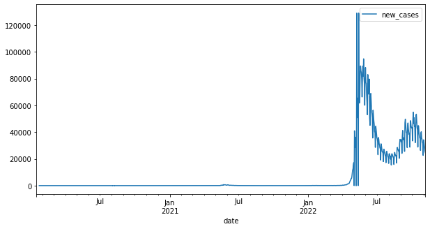
df_tw.plot(x="date", y="new_cases", figsize=(10, 5))
<AxesSubplot:xlabel='date'>
Plot multiple lines#
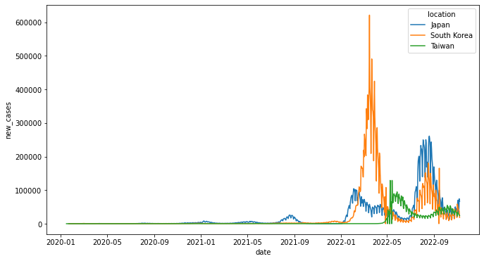
要繪製單一變項(一個國家)的折線圖很容易,X軸為日期、Y軸為案例數。但要如何繪製多個國家、多條折線圖(每個國家一條線)?以下就以日本和台灣兩國的數據為例來進行繪製。
location這個欄位紀錄了該列資料屬於日本或台灣。通常視覺化軟體會有兩種作法,一種做法是必須把日本和台灣在欄的方向展開(用df.pivot()),變成兩個變項,日本和台灣各一個變項,Python最基本的繪圖函式庫matplotlib就必須這麼做。但如果用號稱是matplotlib的進階版seaborn,則可以指定location這個變項作為群組資訊,簡單地說是用location當成群組變數來繪製不同的線。
df1 = df_asia.loc[df_asia['location'].isin(["Taiwan", "Japan"])]
df1['date'] = pd.to_datetime(df1['date'], format="%Y-%m-%d")
set(df1.location)
/var/folders/0p/7xy1_dzx0_s5rnf06c0b316w0000gn/T/ipykernel_38668/2904734101.py:2: SettingWithCopyWarning:
A value is trying to be set on a copy of a slice from a DataFrame.
Try using .loc[row_indexer,col_indexer] = value instead

See the caveats in the documentation: https://pandas.pydata.org/pandas-docs/stable/user_guide/indexing.html#returning-a-view-versus-a-copy
  df1['date'] = pd.to_datetime(df1['date'], format="%Y-%m-%d")
{'Japan', 'Taiwan'}
df1[['location', 'date', 'new_cases']]
| location | date | new_cases | |
|---|---|---|---|
| 104856 | Japan | 2020-01-22 | NaN |
| 104857 | Japan | 2020-01-23 | 0.0 |
| 104858 | Japan | 2020-01-24 | 0.0 |
| 104859 | Japan | 2020-01-25 | 0.0 |
| 104860 | Japan | 2020-01-26 | 2.0 |
| ... | ... | ... | ... |
| 204107 | Taiwan | 2022-11-02 | 33156.0 |
| 204108 | Taiwan | 2022-11-03 | 29952.0 |
| 204109 | Taiwan | 2022-11-04 | 27581.0 |
| 204110 | Taiwan | 2022-11-05 | 25535.0 |
| 204111 | Taiwan | 2022-11-06 | 24345.0 |
2046 rows × 3 columns
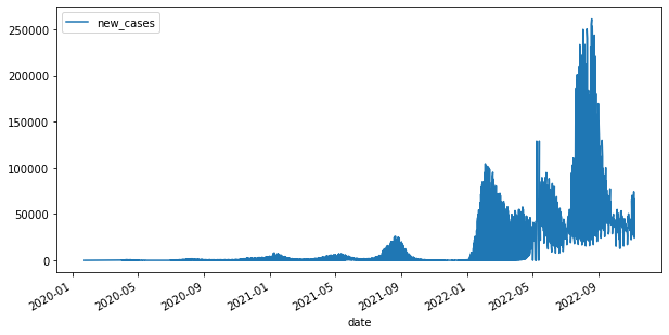
# df1 data contains more than 1 location

df1.plot(x="date", y="new_cases", figsize=(10, 5))
<AxesSubplot:xlabel='date'>
df_wide = df1.pivot(index="date", columns="location",
                    values=["new_cases", "total_cases", "total_vaccinations_per_hundred"])
df_wide
| new_cases | total_cases | total_vaccinations_per_hundred | ||||
|---|---|---|---|---|---|---|
| location | Japan | Taiwan | Japan | Taiwan | Japan | Taiwan |
| date | ||||||
| 2020-01-16 | NaN | NaN | NaN | NaN | NaN | NaN |
| 2020-01-17 | NaN | NaN | NaN | NaN | NaN | NaN |
| 2020-01-18 | NaN | NaN | NaN | NaN | NaN | NaN |
| 2020-01-19 | NaN | NaN | NaN | NaN | NaN | NaN |
| 2020-01-20 | NaN | NaN | NaN | NaN | NaN | NaN |
| ... | ... | ... | ... | ... | ... | ... |
| 2022-11-02 | 70396.0 | 33156.0 | 22460268.0 | 7780125.0 | 268.25 | 264.69 |
| 2022-11-03 | 67473.0 | 29952.0 | 22527741.0 | 7810077.0 | 268.34 | 264.83 |
| 2022-11-04 | 34064.0 | 27581.0 | 22561805.0 | 7837658.0 | 268.56 | 265.00 |
| 2022-11-05 | 74170.0 | 25535.0 | 22635975.0 | 7863193.0 | 268.81 | NaN |
| 2022-11-06 | 66397.0 | 24345.0 | 22702372.0 | 7887538.0 | 268.90 | 265.15 |
1026 rows × 6 columns
fillna()#
df_wide.fillna(0, inplace=True)
df_wide.new_cases.Taiwan
df_wide
| new_cases | total_cases | total_vaccinations_per_hundred | ||||
|---|---|---|---|---|---|---|
| location | Japan | Taiwan | Japan | Taiwan | Japan | Taiwan |
| date | ||||||
| 2020-01-16 | 0.0 | 0.0 | 0.0 | 0.0 | 0.00 | 0.00 |
| 2020-01-17 | 0.0 | 0.0 | 0.0 | 0.0 | 0.00 | 0.00 |
| 2020-01-18 | 0.0 | 0.0 | 0.0 | 0.0 | 0.00 | 0.00 |
| 2020-01-19 | 0.0 | 0.0 | 0.0 | 0.0 | 0.00 | 0.00 |
| 2020-01-20 | 0.0 | 0.0 | 0.0 | 0.0 | 0.00 | 0.00 |
| ... | ... | ... | ... | ... | ... | ... |
| 2022-11-02 | 70396.0 | 33156.0 | 22460268.0 | 7780125.0 | 268.25 | 264.69 |
| 2022-11-03 | 67473.0 | 29952.0 | 22527741.0 | 7810077.0 | 268.34 | 264.83 |
| 2022-11-04 | 34064.0 | 27581.0 | 22561805.0 | 7837658.0 | 268.56 | 265.00 |
| 2022-11-05 | 74170.0 | 25535.0 | 22635975.0 | 7863193.0 | 268.81 | 0.00 |
| 2022-11-06 | 66397.0 | 24345.0 | 22702372.0 | 7887538.0 | 268.90 | 265.15 |
1026 rows × 6 columns
reset_index()#
https://pandas.pydata.org/docs/reference/api/pandas.DataFrame.reset_index.html
在經過pivot後,列方向會變成以date為index,此時我希望將data恢復為欄方向的變數,就需要用reset_index()。
df_wide.reset_index(inplace=True)
df_wide
| date | new_cases | total_cases | total_vaccinations_per_hundred | ||||
|---|---|---|---|---|---|---|---|
| location | Japan | Taiwan | Japan | Taiwan | Japan | Taiwan | |
| 0 | 2020-01-16 | 0.0 | 0.0 | 0.0 | 0.0 | 0.00 | 0.00 |
| 1 | 2020-01-17 | 0.0 | 0.0 | 0.0 | 0.0 | 0.00 | 0.00 |
| 2 | 2020-01-18 | 0.0 | 0.0 | 0.0 | 0.0 | 0.00 | 0.00 |
| 3 | 2020-01-19 | 0.0 | 0.0 | 0.0 | 0.0 | 0.00 | 0.00 |
| 4 | 2020-01-20 | 0.0 | 0.0 | 0.0 | 0.0 | 0.00 | 0.00 |
| ... | ... | ... | ... | ... | ... | ... | ... |
| 1021 | 2022-11-02 | 70396.0 | 33156.0 | 22460268.0 | 7780125.0 | 268.25 | 264.69 |
| 1022 | 2022-11-03 | 67473.0 | 29952.0 | 22527741.0 | 7810077.0 | 268.34 | 264.83 |
| 1023 | 2022-11-04 | 34064.0 | 27581.0 | 22561805.0 | 7837658.0 | 268.56 | 265.00 |
| 1024 | 2022-11-05 | 74170.0 | 25535.0 | 22635975.0 | 7863193.0 | 268.81 | 0.00 |
| 1025 | 2022-11-06 | 66397.0 | 24345.0 | 22702372.0 | 7887538.0 | 268.90 | 265.15 |
1026 rows × 7 columns
Visualized by matplotlib with pandas#
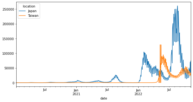
後面加上figsize參數可以調整長寬比。
pandas.DataFrame.plot的可用參數可見https://pandas.pydata.org/docs/reference/api/pandas.DataFrame.plot.html。
df_wide.plot(x="date", y="new_cases", figsize=(10, 5))
<AxesSubplot:xlabel='date'>
More params#
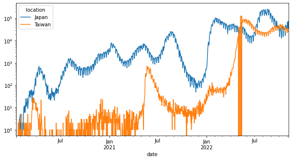
例如對Y軸取log。
pandas.DataFrame.plot的可用參數可見https://pandas.pydata.org/docs/reference/api/pandas.DataFrame.plot.html。
df_wide.plot(x="date", y="new_cases", figsize=(10, 5), logy=True)
<AxesSubplot:xlabel='date'>
Visualized by seaborn#
seaborn可以將location作為群組變數,不同組的就繪製在不同的線。
以下先將location、date、new_cases取出後,把NA值填0。
df1 = df_asia.loc[df_asia['location'].isin(["Taiwan", "Japan", "South Korea"])]
df1['date'] = pd.to_datetime(df1['date'], format="%Y-%m-%d")
df_sns = df1[["location", 'date', 'new_cases']].fillna(0)
df_sns
/var/folders/0p/7xy1_dzx0_s5rnf06c0b316w0000gn/T/ipykernel_38668/2059310855.py:2: SettingWithCopyWarning:
A value is trying to be set on a copy of a slice from a DataFrame.
Try using .loc[row_indexer,col_indexer] = value instead

See the caveats in the documentation: https://pandas.pydata.org/pandas-docs/stable/user_guide/indexing.html#returning-a-view-versus-a-copy
  df1['date'] = pd.to_datetime(df1['date'], format="%Y-%m-%d")
| location | date | new_cases | |
|---|---|---|---|
| 104856 | Japan | 2020-01-22 | 0.0 |
| 104857 | Japan | 2020-01-23 | 0.0 |
| 104858 | Japan | 2020-01-24 | 0.0 |
| 104859 | Japan | 2020-01-25 | 0.0 |
| 104860 | Japan | 2020-01-26 | 2.0 |
| ... | ... | ... | ... |
| 204107 | Taiwan | 2022-11-02 | 33156.0 |
| 204108 | Taiwan | 2022-11-03 | 29952.0 |
| 204109 | Taiwan | 2022-11-04 | 27581.0 |
| 204110 | Taiwan | 2022-11-05 | 25535.0 |
| 204111 | Taiwan | 2022-11-06 | 24345.0 |
3066 rows × 3 columns
Seaborn繪圖還是基於matplotlib套件,但他的lineplot()可以多給一個參數hue,並將location指定給該參數,這樣繪圖時便會依照不同的location進行繪圖。
import matplotlib.pyplot as plt
import seaborn as sns
fig, ax = plt.subplots(figsize=(11, 6))
sns.lineplot(data=df_sns, x='date', y='new_cases', hue='location', ax=ax)
<AxesSubplot:xlabel='date', ylabel='new_cases'>
Visualized by bokeh: plot_bokeh()#
https://towardsdatascience.com/beautiful-and-easy-plotting-in-python-pandas-bokeh-afa92d792167
https://patrikhlobil.github.io/Pandas-Bokeh/ (Document of Pandas-Bokeh)
Bokeh的功能則是可以提供可互動的視覺化。但他不吃Pandas的MultiIndex,所以要將Pandas的階層欄位扁平化。以下是其中一種做法。做完扁平化就可以使用bokeh的函數來進行繪圖。
from bokeh.plotting import figure, show
from bokeh.io import output_notebook
# !pip install pandas_bokeh
import pandas_bokeh
pandas_bokeh.output_notebook()
Collecting pandas_bokeh
  Downloading pandas_bokeh-0.5.5-py2.py3-none-any.whl (29 kB)
Requirement already satisfied: bokeh>=2.0 in /Users/jirlong/opt/anaconda3/lib/python3.9/site-packages (from pandas_bokeh) (2.4.2)
Requirement already satisfied: pandas>=0.22.0 in /Users/jirlong/opt/anaconda3/lib/python3.9/site-packages (from pandas_bokeh) (1.4.2)
Requirement already satisfied: packaging>=16.8 in /Users/jirlong/opt/anaconda3/lib/python3.9/site-packages (from bokeh>=2.0->pandas_bokeh) (21.3)
Requirement already satisfied: tornado>=5.1 in /Users/jirlong/opt/anaconda3/lib/python3.9/site-packages (from bokeh>=2.0->pandas_bokeh) (6.1)
Requirement already satisfied: pillow>=7.1.0 in /Users/jirlong/opt/anaconda3/lib/python3.9/site-packages (from bokeh>=2.0->pandas_bokeh) (9.0.1)
Requirement already satisfied: Jinja2>=2.9 in /Users/jirlong/opt/anaconda3/lib/python3.9/site-packages (from bokeh>=2.0->pandas_bokeh) (2.11.3)
Requirement already satisfied: PyYAML>=3.10 in /Users/jirlong/opt/anaconda3/lib/python3.9/site-packages (from bokeh>=2.0->pandas_bokeh) (6.0)
Requirement already satisfied: typing-extensions>=3.10.0 in /Users/jirlong/opt/anaconda3/lib/python3.9/site-packages (from bokeh>=2.0->pandas_bokeh) (4.1.1)
Requirement already satisfied: numpy>=1.11.3 in /Users/jirlong/opt/anaconda3/lib/python3.9/site-packages (from bokeh>=2.0->pandas_bokeh) (1.21.5)
Requirement already satisfied: MarkupSafe>=0.23 in /Users/jirlong/opt/anaconda3/lib/python3.9/site-packages (from Jinja2>=2.9->bokeh>=2.0->pandas_bokeh) (2.0.1)
Requirement already satisfied: pyparsing!=3.0.5,>=2.0.2 in /Users/jirlong/opt/anaconda3/lib/python3.9/site-packages (from packaging>=16.8->bokeh>=2.0->pandas_bokeh) (3.0.4)
Requirement already satisfied: python-dateutil>=2.8.1 in /Users/jirlong/opt/anaconda3/lib/python3.9/site-packages (from pandas>=0.22.0->pandas_bokeh) (2.8.2)
Requirement already satisfied: pytz>=2020.1 in /Users/jirlong/opt/anaconda3/lib/python3.9/site-packages (from pandas>=0.22.0->pandas_bokeh) (2021.3)
Requirement already satisfied: six>=1.5 in /Users/jirlong/opt/anaconda3/lib/python3.9/site-packages (from python-dateutil>=2.8.1->pandas>=0.22.0->pandas_bokeh) (1.16.0)
Installing collected packages: pandas-bokeh
Successfully installed pandas-bokeh-0.5.5
df_wide2 = df_wide.copy()
df_wide2.columns = df_wide.columns.map('_'.join)
df_wide2
| date_ | new_cases_Japan | new_cases_Taiwan | total_cases_Japan | total_cases_Taiwan | total_vaccinations_per_hundred_Japan | total_vaccinations_per_hundred_Taiwan | |
|---|---|---|---|---|---|---|---|
| 0 | 2020-01-16 | 0.0 | 0.0 | 0.0 | 0.0 | 0.00 | 0.00 |
| 1 | 2020-01-17 | 0.0 | 0.0 | 0.0 | 0.0 | 0.00 | 0.00 |
| 2 | 2020-01-18 | 0.0 | 0.0 | 0.0 | 0.0 | 0.00 | 0.00 |
| 3 | 2020-01-19 | 0.0 | 0.0 | 0.0 | 0.0 | 0.00 | 0.00 |
| 4 | 2020-01-20 | 0.0 | 0.0 | 0.0 | 0.0 | 0.00 | 0.00 |
| ... | ... | ... | ... | ... | ... | ... | ... |
| 1021 | 2022-11-02 | 70396.0 | 33156.0 | 22460268.0 | 7780125.0 | 268.25 | 264.69 |
| 1022 | 2022-11-03 | 67473.0 | 29952.0 | 22527741.0 | 7810077.0 | 268.34 | 264.83 |
| 1023 | 2022-11-04 | 34064.0 | 27581.0 | 22561805.0 | 7837658.0 | 268.56 | 265.00 |
| 1024 | 2022-11-05 | 74170.0 | 25535.0 | 22635975.0 | 7863193.0 | 268.81 | 0.00 |
| 1025 | 2022-11-06 | 66397.0 | 24345.0 | 22702372.0 | 7887538.0 | 268.90 | 265.15 |
1026 rows × 7 columns
df_wide2.plot_bokeh(
    kind='line',
    x='date_',
    y=['new_cases_Japan', 'new_cases_Taiwan']
)
Bar chart: vaccinating rate#
df_asia.dtypes
iso_code                                    object
continent                                   object
location                                    object
date                                        object
total_cases                                float64
                                            ...
population                                 float64
excess_mortality_cumulative_absolute       float64
excess_mortality_cumulative                float64
excess_mortality                           float64
excess_mortality_cumulative_per_million    float64
Length: 67, dtype: object
df_asia['date'] = pd.to_datetime(df_asia.date)
print(df_asia.date.dtype)
datetime64[ns]
/var/folders/0p/7xy1_dzx0_s5rnf06c0b316w0000gn/T/ipykernel_38668/1918172663.py:1: SettingWithCopyWarning:
A value is trying to be set on a copy of a slice from a DataFrame.
Try using .loc[row_indexer,col_indexer] = value instead

See the caveats in the documentation: https://pandas.pydata.org/pandas-docs/stable/user_guide/indexing.html#returning-a-view-versus-a-copy
  df_asia['date'] = pd.to_datetime(df_asia.date)
max(df_asia.date)
Timestamp('2022-11-07 00:00:00')
import datetime
df_recent = df_asia.loc[df_asia['date'] == datetime.datetime(2021, 10, 28)]
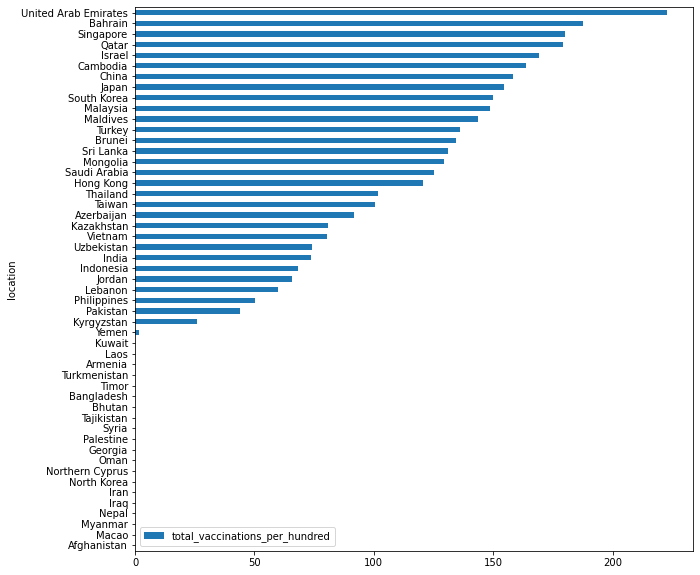
by pure pandas#
# df_recent.columns
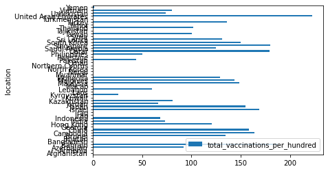
df_recent.plot.barh(x="location", y="total_vaccinations_per_hundred")
<AxesSubplot:ylabel='location'>
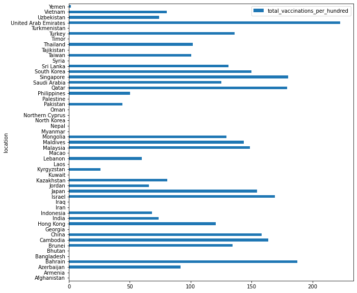
df_recent.plot.barh(x="location", y="total_vaccinations_per_hundred", figsize=(10, 10))
<AxesSubplot:ylabel='location'>
df_recent.sort_values('total_vaccinations_per_hundred', ascending=True).plot.barh(x="location", y="total_vaccinations_per_hundred", figsize=(10, 10))
<AxesSubplot:ylabel='location'>
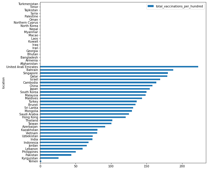
df_recent.fillna(0).sort_values('total_vaccinations_per_hundred', ascending=True).plot.barh(x="location", y="total_vaccinations_per_hundred", figsize=(10, 10))
<AxesSubplot:ylabel='location'>
by plot_bokeh#
toplot = df_recent.fillna(0).sort_values('total_vaccinations_per_hundred', ascending=True)
toplot.plot_bokeh(kind="barh", x="location", y="total_vaccinations_per_hundred")
Bokeh Settings#
Displaying output in jupyter notebook#
Adjust figure size along with windows size#
plot_df = pd.DataFrame({"x":[1, 2, 3, 4, 5],
                        "y":[1, 2, 3, 4, 5],
                        "freq":[10, 20, 13, 40, 35],
                        "label":["10", "20", "13", "40", "35"]})
plot_df
| x | y | freq | label | |
|---|---|---|---|---|
| 0 | 1 | 1 | 10 | 10 |
| 1 | 2 | 2 | 20 | 20 |
| 2 | 3 | 3 | 13 | 13 |
| 3 | 4 | 4 | 40 | 40 |
| 4 | 5 | 5 | 35 | 35 |
p = figure(title = "TEST")
p.circle(plot_df["x"], plot_df["y"], fill_alpha=0.2, size=plot_df["freq"])
p.sizing_mode = 'scale_width'
show(p)
Color mapper#
Categorical color transforming Manually#
# from bokeh.palettes import Magma, Inferno, Plasma, Viridis, Cividis, d3

# cluster_label = list(Counter(df2plot.cluster).keys())
# color_mapper = CategoricalColorMapper(palette=d3['Category20'][len(cluster_label)], factors=cluster_label)
# p = figure(title = "doc clustering")
# p.sizing_mode = 'scale_width'
# p.circle(x = "x", y = "y",
#          color={'field': 'cluster', 'transform': color_mapper},
#          source = df2plot,
#          fill_alpha=0.5, size=5, line_color=None)
# show(p)
Continuous color transforming#
from bokeh.palettes import Magma, Inferno, Plasma, Viridis, Cividis, d3
from bokeh.models import LogColorMapper, LinearColorMapper, LabelSet, ColumnDataSource


p = figure(title = "ColorMapper Tester")
color_mapper = LinearColorMapper(palette="Plasma256",
                                 low = min(plot_df["freq"]),
                                 high = max(plot_df["freq"]))

source = ColumnDataSource(plot_df)
p.circle("x", "y", fill_alpha = 0.5,
         size = "freq",
         line_color=None,
         source = source,
         fill_color = {'field': 'freq', 'transform': color_mapper}
        )

p.sizing_mode = 'scale_width'

show(p)